library(ggplot2)해당 자료는 전북대학교 이영미 교수님 2023응용통계학 자료임
가변수
Example
dt <- data.frame(
  y = c(17,26,21,30,22,1,12,19,4,16,
        28,15,11,38,31,21,20,13,30,14),
  x1 = c(151,92,175,31,104,277,210,120,290,238,
         164,272,295,68,85,224,166,305,124,246),
  x2 = rep(c('M','F'), each=10)
)head(dt)| y | x1 | x2 | |
|---|---|---|---|
| <dbl> | <dbl> | <chr> | |
| 1 | 17 | 151 | M |
| 2 | 26 | 92 | M |
| 3 | 21 | 175 | M |
| 4 | 30 | 31 | M |
| 5 | 22 | 104 | M |
| 6 | 1 | 277 | M |
모든 데이터 퉁으로
model_1 <- lm(y~x1, dt)
summary(model_1)
Call:
lm(formula = y ~ x1, data = dt)

Residuals:
   Min     1Q Median     3Q    Max
-9.579 -4.737  0.721  4.224  7.936

Coefficients:
            Estimate Std. Error t value Pr(>|t|)
(Intercept) 36.40361    2.78580  13.068 1.26e-10 ***
x1          -0.09323    0.01396  -6.677 2.91e-06 ***
---
Signif. codes:  0 ‘***’ 0.001 ‘**’ 0.01 ‘*’ 0.05 ‘.’ 0.1 ‘ ’ 1

Residual standard error: 5.124 on 18 degrees of freedom
Multiple R-squared:  0.7124,    Adjusted R-squared:  0.6964
F-statistic: 44.58 on 1 and 18 DF,  p-value: 2.906e-06
모형은 유의하다.
MSE=5.124
ggplot(dt, aes(x1, y)) +
  geom_point() +
  geom_abline(slope = coef(model_1)[2],
              intercept = coef(model_1)[1], col= 'darkorange')+
  theme_bw()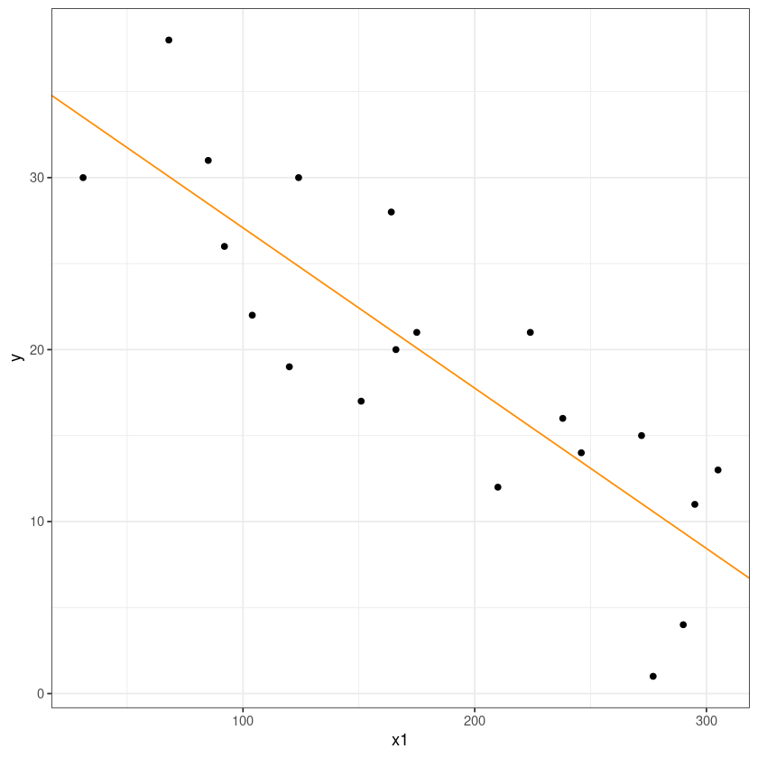
M,F상관없이 모든 데이터 퉁으로!!
\(\widehat y = 36.40361-0.09323 x_1\)
시험성적 1점 올라갈때마다 시간이 0.0932 감소한다.
성별 M,F
model_2 : \(y=\beta_0+\beta_1x_1+\beta_2x_2+\epsilon\)
\(x_2=0 \ if F, x_2=1 \ if M\)
\(E(y|F) : \beta_0 + \beta_1x_1\) 여자가 기준
\(E(y|M) : \beta_0+\beta_1x_1 + \beta_2 = (\beta_0+\beta_2)+\beta_1x_1\)
\(\beta_2 = E(y|M)-E(y|F) = \beta_0 + \beta_2 + \beta_1x_1 - {\beta_0+\beta_1x_1}\)
즉, \(\beta_2\)는 시험성적이 동일할 때 여자와 남자의 소요시간의 평균의 차이
contrasts(factor(dt$x2))| M | |
|---|---|
| F | 0 |
| M | 1 |
\(x_2\)를 factor로 인식했을 때 무엇이 0이고 무엇이 1인지 알려준다.
\(H_0: \beta_1=\beta_2=0\)
################################
# x2 = factor(rep(c('M','F'), each=10)) 로 입력한 경우
#y = b0 + b1x1 + b2x2
# x2 = 0,  F
# x2 = 1,  M
#E(y|M) : b0 + b1x1 + b2 = (b0 + b2) + b1x1
#E(y|F) : b0 + b1x1

# x2 = factor(rep(c(0,1), each=10))로 입력한 경우
# y = b0 + b1x1 + b2x2
# x2 = 0,  M
# x2 = 1,  F
#E(y|M) : b0 + b1x1
#E(y|F) : b0 + b1x1+ b2 = = (b0 + b2) + b1x1


model_2 <- lm(y~x1+x2, dt)
summary(model_2)
Call:
lm(formula = y ~ x1 + x2, data = dt)

Residuals:
    Min      1Q  Median      3Q     Max
-5.0165 -1.7450 -0.6055  1.8803  6.1835

Coefficients:
             Estimate Std. Error t value Pr(>|t|)
(Intercept) 41.768865   1.948930  21.432 9.64e-14 ***
x1          -0.100918   0.008621 -11.707 1.47e-09 ***
x2M         -7.933953   1.414702  -5.608 3.13e-05 ***
---
Signif. codes:  0 ‘***’ 0.001 ‘**’ 0.01 ‘*’ 0.05 ‘.’ 0.1 ‘ ’ 1

Residual standard error: 3.123 on 17 degrees of freedom
Multiple R-squared:  0.8991,    Adjusted R-squared:  0.8872
F-statistic: 75.72 on 2 and 17 DF,  p-value: 3.42e-09
p-value가 유의하다.
model1보다 \(R^2\)값이 많이 올랐다.
model1보다 MSE보다 감소했다.
x2M: x2가 남자 그룹에 있는 계수, F=0이고 M=1이라는 것을 알려준다.\(\beta_2=-7.933953\) 값이 나오는데 강의록에는 F=1,M=0이여서 강의록과는 부호가 바뀐것.
ggplot(dt, aes(x1, y, col=x2)) +
  geom_point() +
  theme_bw() +
  geom_abline(slope = coef(model_2)[2],
              intercept = coef(model_2)[1], col= 'darkorange')+
  geom_abline(slope = coef(model_2)[2],
              intercept = coef(model_2)[1]+coef(model_2)[3], col= 'steelblue')+
  guides(col=guide_legend(title="성별")) +
  scale_color_manual(labels = c("여자", "남자"), values = c("darkorange", "steelblue"))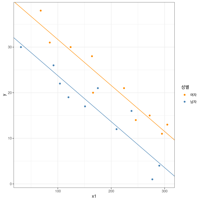
- \(H_0:\beta_2=0 \ vs. \ H_1:\beta_2 \neq 0\)
summary(model_2)$coefficients| Estimate | Std. Error | t value | Pr(>|t|) | |
|---|---|---|---|---|
| (Intercept) | 41.7688646 | 1.948929636 | 21.431694 | 9.640000e-14 |
| x1 | -0.1009177 | 0.008620641 | -11.706522 | 1.468240e-09 |
| x2M | -7.9339526 | 1.414702366 | -5.608213 | 3.134533e-05 |
개별회귀계수에 대한 유의성검정 , 유의확률 값이 작으므로 \(\beta_2=0\)이라고 할 수 있다.
Pr(>|t|)은 양측검정에 대한 유의확률 값이다.\(H_0:\beta_2=0 \ vs. \ H_1:\beta_2 < 0\)
이 때의 유의확률? -> 위의 표와 t-value는 똑같다.
-5.608213\(t=\dfrac{\widehat \beta_2}{\widehat{s.e}(\widehat \beta_2)}\)
H_1:\beta_2 < 0단측 검정에 대한 유의확률 값은Pr(>|t|)/2t-value의
-5.608213값을 제곱하면 아래 표의 F값31.45206이 나온다.Pr(>F)값은 똑같음
-5.608213^2
-31.452053053369
- 자유도가 1개일때 t-value와 F검정의 값은 동일하다
anova(model_1, model_2)| Res.Df | RSS | Df | Sum of Sq | F | Pr(>F) | |
|---|---|---|---|---|---|---|
| <dbl> | <dbl> | <dbl> | <dbl> | <dbl> | <dbl> | |
| 1 | 18 | 472.5913 | NA | NA | NA | NA |
| 2 | 17 | 165.8145 | 1 | 306.7768 | 31.45206 | 3.134533e-05 |
RM: model_1
FM: model_2
472.5913: \(SSE_{RM}\)165.8145: \(SSE_{FM}\)
교호작용
\(y=\beta_0+\beta_1x_1+\beta_2x_2+\beta_3x_1x_2+\epsilon\)
\(x_2 = 0 if F, x_2 = 1 if M\)
\(E(y|F): \beta_0 + \beta_1 x_1\)
\(E(y|M): \beta_0 + \beta_1x_1 + \beta_2 + \beta_3 x_1 = (\beta_0+\beta_2) + (\beta_1+\beta_3)x_1\)
model_3 <- lm(y~x1*x2, dt) #교호작용 보고 싶을 떈 x1*x2 곱하기
# 혹은 lm(y~x1+x2+x1:x2,dt)
summary(model_3)
Call:
lm(formula = y ~ x1 * x2, data = dt)

Residuals:
    Min      1Q  Median      3Q     Max
-5.0463 -1.7591 -0.6232  1.9311  6.1102

Coefficients:
             Estimate Std. Error t value Pr(>|t|)
(Intercept) 41.969620   2.635580  15.924 3.11e-11 ***
x1          -0.101948   0.012474  -8.173 4.20e-07 ***
x2M         -8.313516   3.541379  -2.348   0.0321 *
x1:x2M       0.002089   0.017766   0.118   0.9078
---
Signif. codes:  0 ‘***’ 0.001 ‘**’ 0.01 ‘*’ 0.05 ‘.’ 0.1 ‘ ’ 1

Residual standard error: 3.218 on 16 degrees of freedom
Multiple R-squared:  0.8992,    Adjusted R-squared:  0.8803
F-statistic: 47.56 on 3 and 16 DF,  p-value: 3.405e-08
모형 자첸는 유의하고,
model2에 비하면 \(R^2\)가 더 감소했다.
\(H_0: \beta_3=0 \ vs. \ H_1:\beta_3 \neq 0\)에서 \(H_0\)기각 못함
## y = b0 + b1x1 + b2x2 + b3x1x2
## M : x2=0 => E(y|M) = b0+b1x1
## F : x2=1 => E(y|F) = b0 + b1x1 + b2 + b3x1
##                    = (b0+b2) + (b1+b3)x1

ggplot(dt, aes(x1, y, col=x2)) +
  geom_point() +
  theme_bw() +
  geom_abline(slope = coef(model_3)[2],
              intercept = coef(model_3)[1], col= 'darkorange')+
  geom_abline(slope = coef(model_3)[2]+coef(model_3)[4],
              intercept = coef(model_3)[1]+coef(model_3)[3], col= 'steelblue')+
  guides(col=guide_legend(title="성별")) +
  scale_color_manual(labels = c("여자", "남자"), values = c("darkorange", "steelblue"))
- \(H_0: \beta_3=0 \ vs. \ H_1:\beta_3 \neq 0\)
summary(model_3)$coefficients| Estimate | Std. Error | t value | Pr(>|t|) | |
|---|---|---|---|---|
| (Intercept) | 41.96961960 | 2.63558045 | 15.9242415 | 3.106803e-11 |
| x1 | -0.10194777 | 0.01247420 | -8.1726893 | 4.198832e-07 |
| x2M | -8.31351564 | 3.54137909 | -2.3475362 | 3.209176e-02 |
| x1:x2M | 0.00208933 | 0.01776597 | 0.1176029 | 9.078460e-01 |
anova(model_2, model_3)| Res.Df | RSS | Df | Sum of Sq | F | Pr(>F) | |
|---|---|---|---|---|---|---|
| <dbl> | <dbl> | <dbl> | <dbl> | <dbl> | <dbl> | |
| 1 | 17 | 165.8145 | NA | NA | NA | NA |
| 2 | 16 | 165.6713 | 1 | 0.1432067 | 0.01383045 | 0.907846 |
\(H_0: \beta_2=\beta_3=0 \ vs. \ H_1: not H_0\) 에서
RM: model_1 (x1), FM: model_3 (x1*x2) 아래표 보자
anova(model_1, model_3)| Res.Df | RSS | Df | Sum of Sq | F | Pr(>F) | |
|---|---|---|---|---|---|---|
| <dbl> | <dbl> | <dbl> | <dbl> | <dbl> | <dbl> | |
| 1 | 18 | 472.5913 | NA | NA | NA | NA |
| 2 | 16 | 165.6713 | 2 | 306.92 | 14.82068 | 0.0002280824 |
472.5913=SSE_RM
165.6713=SSE_FM
2=3-1
가변수가 아닌 one-hot encodeing
dt2 <- data.frame(y=dt$y,
                  x1=dt$x1,
                  x2=as.numeric(dt$x2=='M'),
                  x3=as.numeric(dt$x2=='F'))
head(dt2)
| y | x1 | x2 | x3 | |
|---|---|---|---|---|
| <dbl> | <dbl> | <dbl> | <dbl> | |
| 1 | 17 | 151 | 1 | 0 |
| 2 | 26 | 92 | 1 | 0 |
| 3 | 21 | 175 | 1 | 0 |
| 4 | 30 | 31 | 1 | 0 |
| 5 | 22 | 104 | 1 | 0 |
| 6 | 1 | 277 | 1 | 0 |
model_4 <-lm(y~., dt2)
summary(model_4)
Call:
lm(formula = y ~ ., data = dt2)

Residuals:
    Min      1Q  Median      3Q     Max
-5.0165 -1.7450 -0.6055  1.8803  6.1835

Coefficients: (1 not defined because of singularities)
             Estimate Std. Error t value Pr(>|t|)
(Intercept) 41.768865   1.948930  21.432 9.64e-14 ***
x1          -0.100918   0.008621 -11.707 1.47e-09 ***
x2          -7.933953   1.414702  -5.608 3.13e-05 ***
x3                 NA         NA      NA       NA
---
Signif. codes:  0 ‘***’ 0.001 ‘**’ 0.01 ‘*’ 0.05 ‘.’ 0.1 ‘ ’ 1

Residual standard error: 3.123 on 17 degrees of freedom
Multiple R-squared:  0.8991,    Adjusted R-squared:  0.8872
F-statistic: 75.72 on 2 and 17 DF,  p-value: 3.42e-09
\(y=\beta_0+\beta_1x_1+\beta_2x_2+\beta_3x_3+\epsilon\)
full Rank가 아니여서 구할 수 없다..
1 = x2(M)+x3(F) 가 되서 full rank가 안되는데 이중 하나를 날리면 된다.
아래 model_5는 절편이 없는 모델을 만들어서 돌려보자
model_5 <- lm(y~0+x1+x2+x3,dt2)
summary(model_5)
Call:
lm(formula = y ~ 0 + x1 + x2 + x3, data = dt2)

Residuals:
    Min      1Q  Median      3Q     Max
-5.0165 -1.7450 -0.6055  1.8803  6.1835

Coefficients:
    Estimate Std. Error t value Pr(>|t|)
x1 -0.100918   0.008621  -11.71 1.47e-09 ***
x2 33.834912   1.758659   19.24 5.64e-13 ***
x3 41.768865   1.948930   21.43 9.64e-14 ***
---
Signif. codes:  0 ‘***’ 0.001 ‘**’ 0.01 ‘*’ 0.05 ‘.’ 0.1 ‘ ’ 1

Residual standard error: 3.123 on 17 degrees of freedom
Multiple R-squared:  0.982, Adjusted R-squared:  0.9788
F-statistic:   309 on 3 and 17 DF,  p-value: 5.047e-15
modle5 : \(y=\beta_1x_1+\beta_2x_2 + \beta_3x_3 + \epsilon\)
\(x_2 = 1 if M, x_2=0 if F\)
\(x_3 = 0 if M, x_3=1 if F\)
\(E(y|M) = \beta_1x_1 + \beta_2\) - (*)
\(E(y|F) = \beta_1 + \beta_3\)
기울기는 동일한데, 절편이 다르다. 잎에서 쓴 모형과 비교해 본다면,
\(E(y|M) = (\beta_0 + \beta_2) + \beta_1x_1\)에서 (*)의 \(\beta_2 = \beta_0+\beta_2\)
Carseats 예시
install.packages("ISLR")Installing package into ‘/home/coco/R/x86_64-pc-linux-gnu-library/4.2’
(as ‘lib’ is unspecified)
library(ISLR)head(Carseats)
dim(Carseats)| Sales | CompPrice | Income | Advertising | Population | Price | ShelveLoc | Age | Education | Urban | US | |
|---|---|---|---|---|---|---|---|---|---|---|---|
| <dbl> | <dbl> | <dbl> | <dbl> | <dbl> | <dbl> | <fct> | <dbl> | <dbl> | <fct> | <fct> | |
| 1 | 9.50 | 138 | 73 | 11 | 276 | 120 | Bad | 42 | 17 | Yes | Yes |
| 2 | 11.22 | 111 | 48 | 16 | 260 | 83 | Good | 65 | 10 | Yes | Yes |
| 3 | 10.06 | 113 | 35 | 10 | 269 | 80 | Medium | 59 | 12 | Yes | Yes |
| 4 | 7.40 | 117 | 100 | 4 | 466 | 97 | Medium | 55 | 14 | Yes | Yes |
| 5 | 4.15 | 141 | 64 | 3 | 340 | 128 | Bad | 38 | 13 | Yes | No |
| 6 | 10.81 | 124 | 113 | 13 | 501 | 72 | Bad | 78 | 16 | No | Yes |
- 400
- 11
• Sales : 판매량 (단위: 1,000)
• Price : 각 지점에서의 카시트 가격
• ShelveLoc : 진열대의 등급 (Bad, Medium, Good)
• Urban :도시 여부 (Yes, No)
• US: 미국 여부 (Yes, No)
판매량을 예측하자.
\(y=\beta_0 + \beta_1x_1 + \beta_2 x_2 + \beta_3 x_3 + \epsilon\)
\(x_1\):Price, \(x_2,x_3\)는 가변수
\(x_2 = 1\), if ShelveLoc = Good, \(x_2=0\), if o.w.
\(x_3 = 1\), if ShelveLoc = Medium, \(x_3=0\), if o.w.
\(E(y|Bad) = \beta_0+\beta_1x_1\) <- base
\(E(y|Med) = \beta_0 + \beta_1x_1+ \beta_3 = (\beta_0+\beta_3)+\beta_1x_1\)
\(E(y|Good) = \beta_0 + \beta_1x_1 + \beta_2 = (\beta_0+\beta_2) + \beta_1x_1\)
fit <- lm(fit<-lm(Sales~Price+ShelveLoc,
                  data=Carseats))
summary(fit)
Call:
lm(formula = fit <- lm(Sales ~ Price + ShelveLoc, data = Carseats))

Residuals:
    Min      1Q  Median      3Q     Max
-5.8229 -1.3930 -0.0179  1.3868  5.0780

Coefficients:
                 Estimate Std. Error t value Pr(>|t|)
(Intercept)     12.001802   0.503447  23.839  < 2e-16 ***
Price           -0.056698   0.004059 -13.967  < 2e-16 ***
ShelveLocGood    4.895848   0.285921  17.123  < 2e-16 ***
ShelveLocMedium  1.862022   0.234748   7.932 2.23e-14 ***
---
Signif. codes:  0 ‘***’ 0.001 ‘**’ 0.01 ‘*’ 0.05 ‘.’ 0.1 ‘ ’ 1

Residual standard error: 1.917 on 396 degrees of freedom
Multiple R-squared:  0.5426,    Adjusted R-squared:  0.5391
F-statistic: 156.6 on 3 and 396 DF, p-value: < 2.2e-16- 교호작용은 보지 않겠따.
contrasts(Carseats$ShelveLoc)| Good | Medium | |
|---|---|---|
| Bad | 0 | 0 |
| Good | 1 | 0 |
| Medium | 0 | 1 |
ggplot(Carseats, aes(Price, Sales, col=ShelveLoc)) +
  geom_point() +
  theme_bw() +
  geom_abline(slope = coef(fit)[2],
              intercept = coef(fit)[1], col= 'darkorange')+
  geom_abline(slope = coef(fit)[2],
              intercept = coef(fit)[1]+coef(fit)[3], col= 'steelblue')+
  geom_abline(slope = coef(fit)[2],
              intercept = coef(fit)[1]+coef(fit)[4], col= 'darkgreen')+
  guides(col=guide_legend(title="ShelveLoc")) +
  scale_color_manual(labels = c("Bad", "Good", "Medium"),
                     values = c("darkorange", "steelblue","darkgreen"))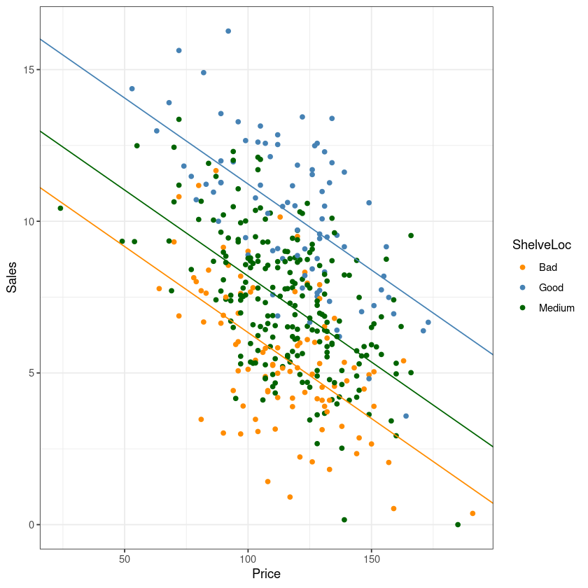
\(y=\beta_0 + \beta_1x_1 + \beta_2 x_2 + \beta_3 x_3 + \beta_4 x_4 \epsilon\)
\(x_2 = 1\), if ShelveLoc = Good, \(x_2=0\), if o.w.
\(x_3 = 1\), if ShelveLoc = Medium, \(x_3=0\), if o.w.
\(x_4 = 1\), if US=yes, \(x_4=0\), if US=no
contrasts(Carseats$US)| Yes | |
|---|---|
| No | 0 |
| Yes | 1 |
fit1 <- lm(fit<-lm(Sales~Price+ShelveLoc+US,
                  data=Carseats))
summary(fit1)
Call:
lm(formula = fit <- lm(Sales ~ Price + ShelveLoc + US, data = Carseats))
Residuals:
Min 1Q Median 3Q Max
-5.1720 -1.2587 -0.0056 1.2815 4.7462
Coefficients:
Estimate Std. Error t value Pr(>|t|)
(Intercept) 11.476347 0.498083 23.041 < 2e-16 ***
Price -0.057825 0.003938 -14.683 < 2e-16 ***
ShelveLocGood 4.827167 0.277294 17.408 < 2e-16 ***
ShelveLocMedium 1.893360 0.227486 8.323 1.42e-15 ***
USYes 1.013071 0.195034 5.194 3.30e-07 ***
---
Signif. codes: 0 ‘***’ 0.001 ‘**’ 0.01 ‘*’ 0.05 ‘.’ 0.1 ‘ ’ 1
Residual standard error: 1.857 on 395 degrees of freedom
Multiple R-squared: 0.5718, Adjusted R-squared: 0.5675
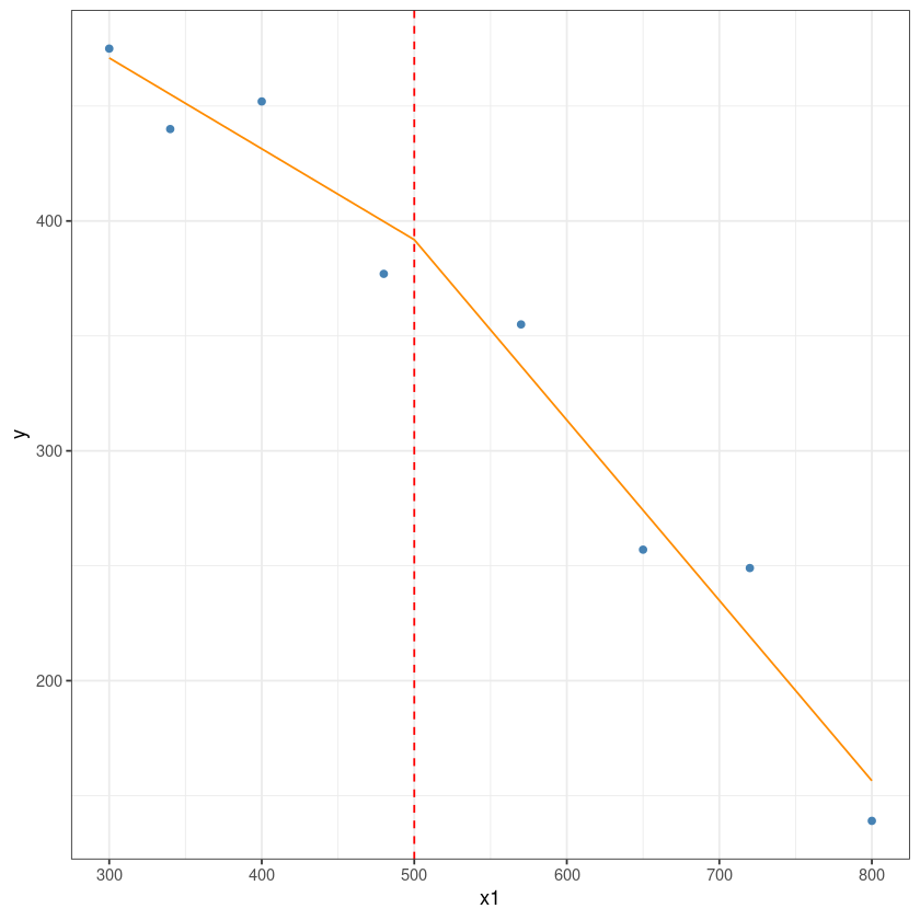
F-statistic: 131.9 on 4 and 395 DF, p-value: < 2.2e-16구간별 회귀분석
dt <- data.frame(
  y = c(377,249,355,475,139,452,440,257),
  x1 = c(480,720,570,300,800,400,340,650)
)ggplot(data = dt, aes(x = x1, y = y)) +
geom_point(color='steelblue') +
theme_bw()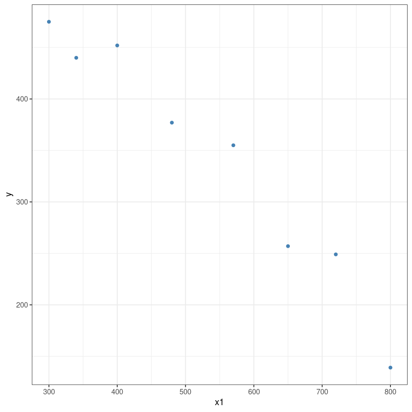
### threshould = 500
## x2(x1-xw)=x2(x1-500) = (x1 - 500)+ := x2

dt$x2 = sapply(dt$x1, function(x) max(0, x-500))
m <- lm(y ~ x1+x2, dt)
summary(m)
Call:
lm(formula = y ~ x1 + x2, data = dt)

Residuals:
      1       2       3       4       5       6       7       8
-22.765  29.765  18.068   4.068 -17.463  20.605 -15.117 -17.160

Coefficients:
            Estimate Std. Error t value Pr(>|t|)
(Intercept) 589.5447    60.4213   9.757 0.000192 ***
x1           -0.3954     0.1492  -2.650 0.045432 *
x2           -0.3893     0.2310  -1.685 0.152774
---
Signif. codes:  0 ‘***’ 0.001 ‘**’ 0.01 ‘*’ 0.05 ‘.’ 0.1 ‘ ’ 1

Residual standard error: 24.49 on 5 degrees of freedom
Multiple R-squared:  0.9693,    Adjusted R-squared:  0.9571
F-statistic: 79.06 on 2 and 5 DF,  p-value: 0.0001645
dt2 <- rbind(dt[,2:3], c(500,0))
dt2$y <- predict(m, newdata = dt2)
# this is the predicted line of multiple linear regression
ggplot(data = dt, aes(x = x1, y = y)) +
geom_point(color='steelblue') +
geom_line(color='darkorange',
data = dt2, aes(x=x1, y=y))+
geom_vline(xintercept = 500, lty=2, col='red')+
theme_bw()